Benton’s Linear/Nonlinear
Logic has
models in (lax) monoidal adjunctions between monoidal and cartesian
categories.
The tasks performed in GPU kernels often deal with linear and
nonlinear maps between real vector spaces.
I want to take this and run with it: let’s see what it looks like to
define some mixed linear/nonlinear functions in a linear/nonlinear
type theory. This feels to me so obvious that it must be written down
somewhere already. In the literature there is work that gets close
(and I’ll do some comparisons at the end), but none are quite what I
want. Please let me know if I’ve missed something.
Edit: It’s been pointed out to me that the type theory I’ve put
together is almost exactly the Enriched Effect
Calculus, though I still
haven’t seen the semantics in ordinary vector spaces discussed
anywhere.
To be totally explicit, what we want to capture is:
Set is cartesian closed with finite coproducts,
VecR is symmetric monoidal closed with finite biproducts.
VecR is powered and copowered over
Set, and in particular there is a lax monoidal adjunction given by
F−U−:≡−⊙R:≡VecR(R,−)
(and F is automatically also strong monoidal by “doctrinal
adjunction”).
There are different presentations of the logic, some which merge the
L and C rules. I want to keep things separated
to avoid (my own) confusion. So we have two term judgements, one
cartesian and one linear.
Γ⊢x:XΓ∣Λ⊢a::A
The context of the linear judgement has two “zones”, with a term such
as the above interpreted as a morphism a:FΓ⊗Λ→A. We don’t need “bunches” in the sense of bunched
logics, because bunching only arises when → and ⊸ exist on
the same mode/category, which is not the case here.
I’ll be consistent about using serif and : for nonlinear
definitions, and sans-serif and :: for linear definitions.Because
linear is bouba and non-linear is kiki.
I will use R to refer to the monoidal unit, although nothing in this
post really requires it to be the real numbers as opposed to an
arbitrary ring. The syntax for the introduction rule e::R is
chosen so that we think of e as an “abstract basis vector”. It
is tempting to use 1 here, but 1 looks more like a constant which
can be dropped into any term in any location, which is certainly not
the case for e.
In most places, I’m going to write functions that involve these
eliminators using pattern matching notation rather than mentioning the
eliminators explicitly. Sue me!
Our first departure from the ordinary presentation of LNL is to
generalise the F and U adjunction to the copower and
“external” hom adjunction
First the copower, a kind of mixed pairing of a nonlinear and linear
type.This kind of mixed paring isn’t novel, a dependent version of
this was used in the LNLD theory of Krishnaswami, Pradic and Benton
(cited below).
We will use this type former to define Rn:≡n⊙R.Though the classical notation Rn does suggest
using the power here… Any time we feel the need to say “pick a
basis for A”, that is a sign we should be using X⊙R instead
(where X can certainly be infinite).
This copower has two different right adjoints, depending on which side
of the ⊙ we transpose. If we transpose the linear side, we get
the nonlinear type of homomorphisms between linear types.Distinct
from the linear type ⊸ of homomorphisms between linear types.
From the above operations we can derive the functors F and
U exactly as suggested earlier: F:≡−⊙R and U:≡VecR(R,−). The derived
rules are slightly different to what you see in other presentations of
LNL, but I think it will help to be explicit about what’s happening to
the unit type R involved in both of these constructions.
For the other right adjoint, if we transpose the nonlinear side of
⊙ we get the power X⋔B. This is the linear type
given by the X-fold product of B with itself.Where does this
pitchfork notation come from originally?
To summarise the four function types we have now:It seems harmless
to have all of these as independent type formers, though you could
define some of them in terms of the others, like VecR(A,B)≅U(A⊸B).
Type Former
Domain
Codomain
Result
−→−
C
C
C
−⊸−
L
L
L
VecR(−,−)
L
L
C
−⋔−
C
L
L
Accordingly, there are four different ways a variable can be bound:
one for each function type. To help distinguish, I’ve used λx
when binding a nonlinear variable, so for → and ⋔, and
∂a when binding a linear variable, so for ⊸ and
Vec(−,−).
We’ll need to be able to eliminate nonlinear inductive types into the
linear term judgement.In Mike’s terminology this is asking that the
mode morphism from nonlinear types into linear ones is “transparent”.
(I think.) This should be derivable because F is a left
adjoint, but it’s convenient to just have it as a rule. For example,
for Bool:
This kind of nonlinear interaction is a change in perspective compared
to other applications of LNL. I don’t want to think of the nonlinear
world as a “metatheory” for building linear maps (like quantum
circuits, say), but as something that can be jumbled together with the
linear type formers.
This is the other feature that goes beyond the original LNL logic: we
add in global “additivity” rules for all linear types. This will
turn the products we just put in above into biproducts.And note also
that “addition is additive”, in that the linear context is not split
into two pieces by the + rule.
Besides being commutative, associative and unital, these global rules
will need to interact sensibly with the other type formers:
(Or in monU we could not pattern match on the unit and
use the argument on one of the sides.)
It’s similarly straightforward to show that all our type formers are
functorial. For purely linear or nonlinear type formers it goes
exactly as normal, so I’ll just demonstrate the ones that involve both
linear and nonlinear types.
Interestingly, there’s a different kind of functoriality for
⋔: nonlinear functoriality on the underlying sets. This is
a genuinely different construction to the above, not just its image
under some bijection, because the provided function could nonlinearly
scramble all the elements of UA.What a mess!
Global additivity gives A&B the universal property of
the coproduct. Let’s just rename the type former to A⊕B from
this point on (though in linear logic this is usually used for the
additive coproduct).
In the latter case, we could do unit-induction on both sides or just
keep it one-sided. We can derelict multiplication to a nonlinear map,
using the same idea as monU:
mult:UR×UR→URmult(a,b):≡∂e.mult(a(e)⊗b(e))
Nonlinearly, we have 1:UR defined as the identity
homomorphism 1:≡∂r.r.
We certainly have 0::R linearly because we put zero in as a rule,
from which we can define ∂r.0:UR. Addition is not
bilinear, so the best we can hope for is a map UR×UR→UR, which we can define using global additivity.
add:UR×UR→URadd(a,b):≡∂r.a(r)+b(r)
At this point it would be sensible to check that the ring axioms hold
for UR, using the equations we put in for +.
Let’s suppose we have (nonlinear) finite types n, which we can
pattern match on and manipulate as normal. Euclidean spaces
Rn are defined by Rn:≡n⊙R, or in
other words, Fn. We can define the dot product as a linear
map, using case analysis on the nonlinear Boolean value of i=j.
Or, if you want to be edgy:In the special case of X⊙R, we
could write the term/pattern (i⊙e) as ei: it really
is like we’re pattern-matching on basis vectors. But I’ll resist doing
that in this post, to make it easier to remember that it’s really
⊙.
dot((i⊙e)⊗(j⊙e)):≡ifi=jtheneelse0
We are usually handed two separate vectors nonlinearly, and like
before we can handle this by dereliction.
dot:URn×URn→URdot(u,v):≡∂e.dot(u(e)⊗v(e))
These definitions generalise easily to matrix multiplication, by
functoriality of ⊗. This is the place where the
linear/nonlinear logic really shines, so let’s hope there’s a lot of
this.
How do we iterate over a vector of real numbers? Realistically, we
probably want iteration over a vector to be a primitiveAs it is in
Futhark, for example., but assuming some
reasonable rules for the finite types n we can do it by
induction.These examples do need proper nonlinear dependent types to
make sense, but hopefully you get the idea. We are doing dependent
elimination on the n:N parameter of the finite type
former.
suggests that we can pattern match on elements of Rn+1 as R⊕RnI’m cheating here, officially we are accessing
elements of A⊕B by projection rather than pattern matching,
but the projection syntax is a bit noisy.. Then, for example:
This kind of induction also lets us give an inverse to
unexplode above:
exploden::(Rn⊸A)⊸(Rn⊗A)explode0(h):≡0exploden+1(h):≡(zero⊙e)⊗h(zero⊙e)+(ι⊗idA)(exploden(h∘ι))
where ι::Rn⊸Rn+1 is the inclusion ι(i⊙e):≡suc(i)⊙e. Nonlinearly:
What does it look like to apply a nonlinear function along an axis?
This can’t be done generically, in the sense of defining a map
map2:(UB→UC)→U(A⊗B)→U(A⊗C)
for an arbitrary linear type A, because the result really does
depend on a choice of basis for A. This is easiest to do if we first
take the inputs in unexploded form.Using X⊙R makes clear
that this function does require us to pick a basis, but doesn’t
require the vector space to be finite dimensional.
Now, if we really want to define map2 as map on (the
underlying set of) the tensor type, we unexplode the matrix into a
homomorphism, compose, and then re-explode:And here, we see that the
final exploding step is the only place we actually need that
Rq is finite dimensional.
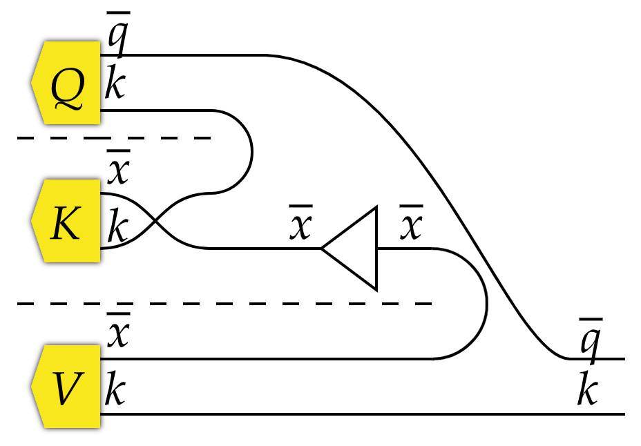
Let’s try to apply what we’ve learned so far to the most famous
linear/nonlinear map of R-vector spaces in the world: the attention
mechanism. Here’s a string diagram of what we’re trying to replicate
in code, where the “caps” represent the dot map from above,
and the triangular node represents softmax:I find these kinds of
“string diagrams” quite confusing, because the interchange law fails
when mixing linear/nonlinear maps and the meaning of a diagram is not
invariant under isotopy. In other words, the relative horizontal
position of the nodes matters; even when the nodes are completely
disconnected from one other. Here, pulling the upper cap past the
softmax results in a different map.
Of course, we can’t fuse this into a single linear map because it
involves the non-linear softmax:URn→UR.We
could define softmax ourselves using iteration, if we assume we
have exp:UR→UR and recip:UR→UR, say. Taken literally, that diagram is
attention:U(Rq⊗Rk)×U(Rx⊗Rk)×U(Rx⊗Rk)→U(Rq⊗Rk)
But we’re better just using VecR everywhere we can, and exploding
things later if we really want:
This is about as simple as we could hope for! It almost looks like we
haven’t done anything at all, but this syntax tracks and enforces the
correct interaction of the linear and nonlinear parts of the
definition. I think this is a good place to stop for now.
One probably wants a version of this that has dependent nonlinear
types, and linear types that can depend on those nonlinear types (but
not on other linear types). If nothing else, we need this to actually
justify the way we used the finite types n. For inspiration
one should probably look at:
[1]
N.
R. Krishnaswami, P. Pradic, and N. Benton, “Integrating
linear and dependent types,” in POPL, 2015, pp.
17–30. doi: 10.1145/2676726.2676969.
There are a couple of similar existing bits of work. Closest is
Jennifer Paykin’s thesis and some of the related papers.
[4]
J.
Paykin, “Linear/non-linear types for embedded
domain-specific languages,” PhD thesis, University of
Pennsylvania, 2018. doi: 20.500.14332/29702.
The thesis demonstrates how to implement LNL as an embedded language
inside a nonlinear host language like Haskell or Coq, and this looks
like it works very well in practice. If I understand right, the focus
is more on using the nonlinear language as a metalanguage for the
linear language, rather than considering the whole system together as
being semantically useful. This is also the case for the Quipper line
of work. Her Box constructor is like the external hom,
which I here called VecR(−,−).
M.
Vákár, “Reverse AD at higher types: Pure, principled and
denotationally correct,” in Programming languages
and systems, Cham: Springer International Publishing, 2021, pp.
607–634.
[7]
M.
Vákár and T. Smeding, “CHAD: Combinatory homomorphic
automatic differentiation,”ACM Trans. Program.
Lang. Syst., vol. 44, no. 3, Aug. 2022, doi: 10.1145/3527634.
[8]
F.
Lucatelli Nunes and M. Vákár, “CHAD for
expressive total languages,”Math. Structures
Comput. Sci., vol. 33, no. 4–5, pp. 311–426, 2023, doi: 10.1017/s096012952300018x.
[9]
T.
J. Smeding and M. I. L. Vákár, “Efficient
CHAD,”Proc. ACM Program. Lang., vol. 8, no.
POPL, Jan. 2024, doi: 10.1145/3632878.
This is exciting work, and the part relevant to us is the
linear/nonlinear “target” language for their source transformation.
Unfortunately the linear context zone in this type theory is a
“stoup”, meaning that it contains exactly one linear variable.If
there’s some CHAD work that I missed which covers the properly linear
tensor product, please let me know! As a result, that language is not
able to express the linear tensor product, which is something I
definitely want to have.
Separately, additivity and the λ-calculus has been considered
in the following line of work:
[11]
A.
Díaz-Caro and G. Dowek, “A linear linear
lambda-calculus,”Mathematical Structures in
Computer Science, vol. 34, no. 10, pp. 1103–1137, 2024, doi: 10.1017/S0960129524000197.
[12]
A.
Díaz-Caro, M. Ivnisky, and O. Malherbe, “An algebraic
extension of intuitionistic linear logic: The L!S-calculus and its categorical
model.” 2025. Available: https://arxiv.org/abs/2504.12128
The first paper considers additivity in the context of the ordinary
lambda calculus, and the second considers additivity in the context of
intuitionistic linear logic but with a dual-zone context structure
different to ours. There are only linear types, with the “nonlinear”
part of the context corresponding to linear types that have had the
! comonad applied. Accordingly, there are no nonlinear type
formers, like functions/products/coproducts etc.
There is also some work on modelling the lambda calculus directly in
finite dimensional vector spaces over finite fields.
[13]
B.
Valiron and S. Zdancewic, “Modeling simply-typed lambda
calculi in the category of finite vector spaces,”Sci. Ann. Comput. Sci., vol. 24, no. 2, pp. 325–368, 2014, doi:
10.7561/SACS.2014.2.325.
Here, the theory being modelled really is the ordinary non-linear
lambda calculus without any linear features, though they do also
consider additivity.
The purpose of both restricting to finite dimensional vector spaces
and finite base fields is so that the comonad !:≡FU (in our notation) is strong monoidal: !(A×B)≅!A⊗!B. This is not a problem for us, because our
priority is matching the semantics in R-vector spaces
rather than matching the linear logic rules for !.